Quantum Processing – Understand the Bernstein-Vazirani algorithm
Posted on Thu 06 August 2026 in quantum
We have seen previously the Bernstein-Vazirani algorithm.
This algorithm is a search algorithm. Given an unknown function \(f\) that returns \(1\) only for a single value \(x\), and \(0\) otherwise, BV Algorithm will find \(x\). Well, \(f\) is not completely unknown. We know it is a dot product of its input with a secret key. But we don't know this secret key.
With classical algorithms, you'll have to test all possibilities. BV algorithm finds \(x\) in a single shot.
To understand how it works, let's go back and take a closer look at the CNOT gate.
Understanding CNOT Gate
To really understand the effect of entanglement and the CNOT gate, let's inspect this small circuit:
import qiskit as q
import qiskit_aer as qaer

def build_circuit():
    # build a quantum circuit with 2 qbits and 1 classical bits
    qc = q.QuantumCircuit(2, 1)

    qc.h(0)
    qc.h(1)
    qc.cx(0, 1) # cx <=> cnot
    qc.h(0)

    qc.measure(0, 0)

    return qc


# Helper function to execute given circuit
def execute(circuit):
    simulator = qaer.AerSimulator(method="statevector")
    qc = q.transpile(circuit, simulator)
    job = simulator.run(qc, memory=True, shots=100)
    result = job.result()
    return result


circuit = build_circuit()
print(circuit)

result = execute(circuit)
print(result.get_counts())
And the result:
     ┌───┐     ┌───┐┌─┐
q_0: ┤ H ├──■──┤ H ├┤M├
     ├───┤┌─┴─┐└───┘└╥┘
q_1: ┤ H ├┤ X ├──────╫─
     └───┘└───┘      ║
c: 1/════════════════╩═
                     0
{'0': 100} <== q_0 = 0
q_0 is a control qubit. If its value is 0, q_1 is not changed. If its value is 1, q_1 is flipped. In the example above, both qubits are initialized at 0. H puts q_0 in superposition, then q_0 is used as a controlled qubit of the CNOT gate, and finally an H gate is applied to q_0 to put it back to a defined state. When measured, its value is 0 100% of the time.
Now, what happens if we modify q_1 ? Instinctively, q_0 has no reason to be modified, as it "controls" q_1, not the other way around, right?...
def build_circuit():
    qc = q.QuantumCircuit(2, 1)

    qc.h(0)
    qc.h(1)
    qc.z(1) # <= add this gate
    qc.cx(0, 1)
    qc.h(0)

    qc.measure(0, 0)

    return qc
     ┌───┐          ┌───┐┌─┐
q_0: ┤ H ├───────■──┤ H ├┤M├
     ├───┤┌───┐┌─┴─┐└───┘└╥┘
q_1: ┤ H ├┤ Z ├┤ X ├──────╫─
     └───┘└───┘└───┘      ║
c: 1/═════════════════════╩═
                          0
{'1': 100} <== q_0 = 1
q_0 is now 1.
— WHAT? What sorcery is it?!!!
Yes. Even if it is called "control qubit", it can be modified by the 2nd qubit. Calling one qubit the "control" and the second the "target" is arbitrary. Since the beginning, we have worked on the \(\{ \left| 0 \right>, \left| 1 \right>\}\) basis, which is represented by the Z axis on the Bloch sphere. But we could work on any orthonormal basis, like \(\{ \left| + \right>, \left| - \right>\}\), which is the X axis. I won't do the math, but you would see that on this basis, the "control" (unchanged) qubit would be the 2nd, and the "target" would be the 1st one. Thus, on this basis, the sense of which bit is the control bit and which the target bit has reversed.
Both qubits are equally affected by the CNOT gate.
— Ohhhhh! Like in Harry Potter!
Wait, what?
— You know, the prophecy. "Neither can live while the other survives".
Yes, if you want.
So both qubits are equally affected by each other, but depending on whether we look at it from the front or from below, one or the other qubit may seem unchanged and the other flipped.
Understanding Bernstein-Vazirani Quantum Algorithm
Given an unknown oracle function, the BV algorithm looks like this:
     ┌───┐      ░ ┌─────┐ ░ ┌───┐┌─┐
q_0: ┤ H ├──────░─┤  O  ├─░─┤ H ├┤M├──────
     ├───┤      ░ │  R  │ ░ ├───┤└╥┘┌─┐
q_1: ┤ H ├──────░─┤  A  ├─░─┤ H ├─╫─┤M├───
     ├───┤      ░ │  C  │ ░ ├───┤ ║ └╥┘┌─┐
q_2: ┤ H ├──────░─┤  L  ├─░─┤ H ├─╫──╫─┤M├
     ├───┤┌───┐ ░ │  E  │ ░ └───┘ ║  ║ └╥┘
q_3: ┤ H ├┤ Z ├─░─┤     ├─░───────╫──╫──╫─
     └───┘└───┘ ░ └─────┘ ░       ║  ║  ║
c: 3/═════════════════════════════╩══╩══╩═
                                  0  1  2
First, all qubits are put in a superposition state. If you remember the Bloch Sphere representation, they all end up like this:
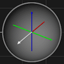
The last one, which contains the result of the oracle, also has a Z gate, which puts it like this:
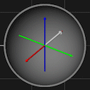
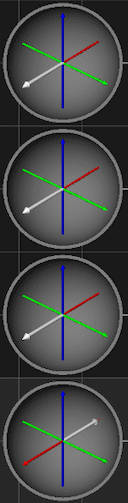
This means the input of the oracle is:
We don't know the secret key encoded in the oracle, but we know how the oracle is implemented. Here are the 8 possible oracles for key \([0, 0, 0], [0, 0, 1], [0, 1, 0], \dots ,[1, 1, 1]\):
─────────────    ───────■───────    ───────────────    ──────■──────────
                        │                                    │
─────────────    ───────┼───────    ───────■───────    ──────┼────■─────
                        │                  │                 │    │
─────────────    ───────┼───────    ───────┼───────    ──────┼────┼─────
                      ┌─┴─┐              ┌─┴─┐             ┌─┴─┐┌─┴─┐
─────────────    ─────┤ X ├─────    ─────┤ X ├─────    ────┤ X ├┤ X ├───
                      └───┘              └───┘             └───┘└───┘


─────────────    ────■──────────    ───────────────    ───■─────────────
                     │                                    │
─────────────    ────┼──────────    ─────■─────────    ───┼────■────────
                     │                   │                │    │
──────■──────    ────┼────■─────    ─────┼────■────    ───┼────┼────■───
    ┌─┴─┐          ┌─┴─┐┌─┴─┐          ┌─┴─┐┌─┴─┐       ┌─┴─┐┌─┴─┐┌─┴─┐
────┤ X ├────    ──┤ X ├┤ X ├───    ───┤ X ├┤ X ├──    ─┤ X ├┤ X ├┤ X ├─
    └───┘          └───┘└───┘          └───┘└───┘       └───┘└───┘└───┘
Not all oracles are implemented this way, but the BV algorithm works only with this kind of oracle.
Let's have a look at the circuit for \([1, 0, 1]\):
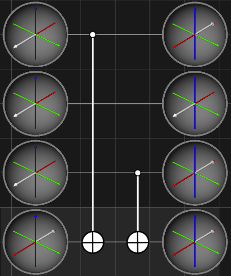
As you may have noticed, the control bits q_0 and q_3 are flipped, because they are influenced by the target bit q_4. q_0 and q_2 are \(\left| - \right>\) and q_1 is \(\left| + \right>\). But there is still one issue. If we do a measurement, we end up with this (1000 shot simulation using qiskit):
     ┌───┐      ░            ░ ┌─┐
q_0: ┤ H ├──────░───■────────░─┤M├──────
     ├───┤      ░   │        ░ └╥┘┌─┐
q_1: ┤ H ├──────░───┼────────░──╫─┤M├───
     ├───┤      ░   │        ░  ║ └╥┘┌─┐
q_2: ┤ H ├──────░───┼────■───░──╫──╫─┤M├
     ├───┤┌───┐ ░ ┌─┴─┐┌─┴─┐ ░  ║  ║ └╥┘
q_3: ┤ H ├┤ Z ├─░─┤ X ├┤ X ├─░──╫──╫──╫─
     └───┘└───┘ ░ └───┘└───┘ ░  ║  ║  ║
c: 3/═══════════════════════════╩══╩══╩═
                                0  1  2
{'000': 113,
 '001': 147,
 '010': 126,
 '011': 127,
 '100': 111,
 '101': 110,
 '110': 140,
 '111': 126}
Meaning after the oracle, every measurement is possible with the same probabilities around \(12\%\). Shit! We cannot differentiate one state from another. That's where the last H gates of the BV circuit come into play. H gates transform a basis state into a superposition state. But they also do the opposite, transforming a superposition state into a basis state. In particular, they transform \(\left| + \right>\) into \(\left| 0 \right>\) and \(\left| - \right>\) into \(\left| 1 \right>\). In other words, they transform a horizontal arrow on the Bloch sphere into a vertical arrow, which can be measured:
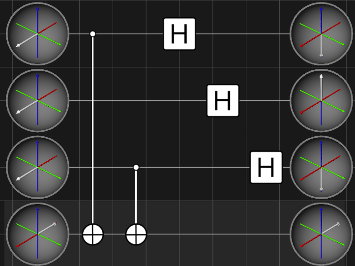
Let's simulate this with Qiskit:
import qiskit as q
import qiskit_aer as qaer


def build_circuit():
    qc = q.QuantumCircuit(4, 3)

    qc.h(0)
    qc.h(1)
    qc.h(2)
    qc.h(3)
    qc.z(3)

    qc.barrier()

    qc.cx(0, 3)
    qc.cx(2, 3)

    qc.barrier()

    qc.h(0)
    qc.h(1)
    qc.h(2)
    qc.measure(0, 0)
    qc.measure(1, 1)
    qc.measure(2, 2)

    return qc


# Helper function to execute given circuit
def execute(circuit):
    simulator = qaer.AerSimulator(method="statevector")
    qc = q.transpile(circuit, simulator)
    job = simulator.run(qc, memory=True, shots=1000)
    result = job.result()
    return result


circuit = build_circuit()
print(circuit)

result = execute(circuit)
print(dict(sorted(result.get_counts().items())))
     ┌───┐      ░            ░ ┌───┐┌─┐
q_0: ┤ H ├──────░───■────────░─┤ H ├┤M├──────
     ├───┤      ░   │        ░ ├───┤└╥┘┌─┐
q_1: ┤ H ├──────░───┼────────░─┤ H ├─╫─┤M├───
     ├───┤      ░   │        ░ ├───┤ ║ └╥┘┌─┐
q_2: ┤ H ├──────░───┼────■───░─┤ H ├─╫──╫─┤M├
     ├───┤┌───┐ ░ ┌─┴─┐┌─┴─┐ ░ └───┘ ║  ║ └╥┘
q_3: ┤ H ├┤ Z ├─░─┤ X ├┤ X ├─░───────╫──╫──╫─
     └───┘└───┘ ░ └───┘└───┘ ░       ║  ║  ║
c: 3/════════════════════════════════╩══╩══╩═
                                     0  1  2
{'101': 1000}
Which means there is \(100\%\) probability of measuring \([1, 0, 1]\), which is our secret key. We just need one execution to find it. The funny thing is that we don't even read q_4, the output of the oracle.
You can try with other oracles as well, or with more qubits.
Takeaways
- CNOT control qubit is influenced by the target qubit.
- Input qubits also carry information about the output of an algorithm.
- H gate can also be used to put a quantum state back in a basis state.